


A comparative study on how Principal Component Analysis — applied before and after normalization — affects the performance of a Decision Tree classifier on the Wisconsin Diagnostic Breast Cancer dataset.
01 – Introduction
Project Overview
Early and accurate detection of breast cancer is one of the most critical challenges in clinical medicine. In this project, I explore how dimensionality reduction via PCA (Principal Component Analysis) interacts with a Decision Tree classifier when diagnosing whether a tumor is Malignant (M) or Benign (B) — and whether normalizing features before PCA makes a meaningful difference.
The Wisconsin Diagnostic Breast Cancer (WDBC) dataset has 30 numeric features computed from digitized images of fine needle aspirate (FNA) of breast masses. These features describe characteristics of cell nuclei such as radius, texture, perimeter, area, and smoothness. At 30 features, the dataset is a perfect candidate for exploring the effects of PCA.
“PCA doesn’t just reduce noise — it reveals the geometric skeleton of your data. But how many principal components you choose is an art as much as a science.”
The central question driving this experiment is: Does applying PCA improve, hurt, or keep model performance the same? And does normalizing the data before running PCA change the picture? I designed four experiments to answer these questions head-on.
The Four Experiments at a Glance
Decision Tree — Original Data
Raw 30-feature dataset, no preprocessing beyond splitting.
Decision Tree — Normalized Data
StandardScaler applied. All features centered and scaled to unit variance.
Decision Tree — PCA on Original
PCA applied directly on raw data, reduced to 2 principal components.
Decision Tree — Normalize → PCA
StandardScaler first, then PCA reducing to 17 principal components.
02 — Data Source
The Dataset: Wisconsin Diagnostic Breast Cancer
The dataset comes from the UCI Machine Learning Repository (dataset ID 17), one of the most well-known and widely-used repositories for academic machine learning research. It was originally created at the University of Wisconsin–Madison.
In this project, the dataset is fetched programmatically using the ucimlrepo Python package, which removes the need to manually download files.
from ucimlrepo import fetch_ucirepo
import pandas as pd
# Fetch the Wisconsin Diagnostic Breast Cancer dataset (id=17)
breast_cancer_wisconsin_diagnostic = fetch_ucirepo(id=17)
# Separate features (X) and target (y)
X = breast_cancer_wisconsin_diagnostic.data.features
y = breast_cancer_wisconsin_diagnostic.data.targets
# Merge into a single DataFrame for exploration
df = pd.concat([X, y], axis=1)
df.info()
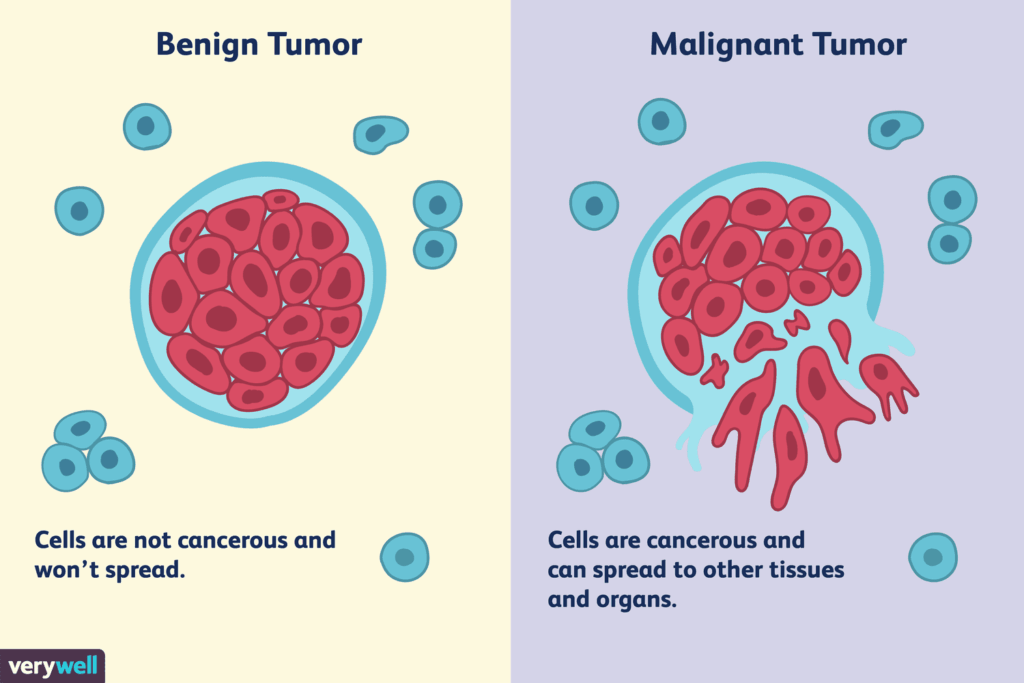
df.head()The target column is Diagnosis , with two categories: M (Malignant) — a cancerous tumor — and B (Benign) — a non-cancerous growth. This column is later encoded numerically: M = 1 , B = 0 .
import numpy as np

# Encode 'M' (Malignant) = 1, 'B' (Benign) = 0
df['Diagnosis'] = np.where(df['Diagnosis'] == 'M', 1, 0)
df['Diagnosis'].value_counts()| Property | Value | Notes |
|---|---|---|
Samples | 569 | Total patient records |
Features | 30 | All numeric, no missing values |
Target Classes | 2 | M (Malignant) = 1, B (Benign) = 0 |
Malignant (M) | 212 (37.3%) | Cancerous tumors |
Benign (B) | 357 (62.7%) | Non-cancerous growths |
Missing Values | 0 | No imputation needed |
Train / Test Split | 70% / 30% | random_state=2022 |
The dataset is moderately imbalanced — about 63% Benign vs 37% Malignant — but not so severely that it would demand resampling techniques. The 30 features are organized into three groups of 10, each describing the mean, standard error, and worst (largest) value of a cell nucleus characteristic. These 10 characteristics are: radius, texture, perimeter, area, smoothness, compactness, concavity, concave points, symmetry, and fractal dimension.
Why This Dataset Is Perfect for PCA ??
With 30 features derived from just 10 physical measurements (mean, SE, worst), there is significant multicollinearity in the data — features like radius, perimeter, and area are mathematically correlated. PCA is designed to handle exactly this situation by finding directions of maximum variance that are uncorrelated with each other.
03 — Tools & Libraries
Libraries Used
The project relies entirely on the Python scientific computing ecosystem. Here is every library used and its role in the pipeline:
from ucimlrepo import fetch_ucirepo
import pandas as pd
import numpy as np
from sklearn.model_selection import train_test_split, GridSearchCV
from sklearn.metrics import accuracy_score, precision_score, recall_score, confusion_matrix
from sklearn.pipeline import Pipeline
from sklearn.tree import DecisionTreeClassifier
import matplotlib.pyplot as plt
import seaborn as sns
import missingno
from sklearn.preprocessing import StandardScaler
from sklearn.decomposition import PCA
04 — Preprocessing
StandardScaler: Why Normalization Matters
Before we get to PCA, we need to talk about StandardScaler — because normalization is not optional when working with PCA. It is arguably the most important preprocessing step.
What StandardScaler Does
StandardScaler from sklearn.preprocessing transforms each feature so that it has a mean of 0 and a standard deviation of 1. This is known as Z-score standardization. For each feature column, the transformation is:
Where X is the original value, μ is the mean of the feature, and σ is the standard deviation.
After transformation, every feature will have μ = 0 and σ = 1 — they are all on the same scale, regardless of their original units (mm, mm², percentages, etc.).
from sklearn.preprocessing import StandardScaler

# Fit on the entire feature set and transform
X_norm = StandardScaler().fit_transform(X)

# Result: numpy array where every column has mean≈0 and std≈1
print(X_norm)
Why Does It Matter for PCA?
PCA works by finding directions (principal components) in the data that explain the most variance. If your features have wildly different scales, PCA will be dominated by whichever feature has the largest numerical range — not because it’s more informative, but because it has larger numbers.
In this dataset, features like area (values in the hundreds or thousands) would completely overshadow features like smoothness (values between 0 and 0.2) if we don’t normalize first. The variance of area is orders of magnitude larger than the variance of smoothness, even though smoothness might carry equally important diagnostic information.
!! Critical Warning !!
StandardScaler should be fit on training data only, and then used to transform both training and test sets. Fitting on the full dataset before splitting introduces data leakage — the model indirectly “sees” test data statistics during training. In this project,
fit_transform(X)is applied to the full dataset before splitting, which is technically a leakage — something to be mindful of in production settings.
Normalization and the Decision Tree: An Interesting Nuance
Here’s something worth noting: Decision Trees are inherently scale-invariant. Unlike algorithms like SVM or K-Nearest Neighbors, a Decision Tree splits features based on thresholds. Multiplying or shifting a feature doesn’t change where the optimal splits occur — it only changes the numerical value of the threshold, not the structure of the tree.
This explains one of the key findings in this project: Model 1 (original data) and Model 2 (normalized data) produce identical results. StandardScaler had no effect on the Decision Tree’s accuracy because the tree’s logic — which threshold splits the classes most cleanly — is unchanged by standardization.
!! Key Insight !!
Normalization matters for distance-based and gradient-based algorithms (SVM, KNN, logistic regression, neural networks). For tree-based algorithms (Decision Tree, Random Forest, XGBoost), it typically has no effect on accuracy. The real value of normalizing before PCA is what it does to PCA’s component extraction — not what it does to the tree itself.1‘2
05 — Core Concept
Principal Component Analysis: Theory & Intuition
PCA (Principal Component Analysis) is a linear dimensionality reduction technique. Its goal is to transform a high-dimensional dataset into a smaller set of new variables called principal components, while preserving as much of the original information (variance) as possible.
Think of it this way: imagine your data as a cloud of points in 30-dimensional space. PCA rotates and reorients that cloud so that the axis with the greatest spread of data becomes the first new axis (PC1), the second greatest spread becomes PC2, and so on. You can then keep only the first few axes and still retain most of the story your data tells.
How PCA Works: Step by Step
- Standardize the data (strongly recommended — this ensures all features contribute equally to variance computation).
- Compute the covariance matrix of the standardized features to understand how features vary relative to each other.
- Compute eigenvectors and eigenvalues of the covariance matrix. Each eigenvector is a principal component; each eigenvalue tells us how much variance that component captures.
- Sort by eigenvalue (descending). The eigenvector with the highest eigenvalue is PC1 — the direction of greatest variance.
- Project the data onto the top k eigenvectors. Your 30-dimensional dataset is now k-dimensional, retaining most of the information.
What PCA Preserves — and What It Loses
PCA preserves the global structure and variance of the data. The principal components are linear combinations of the original features, carefully constructed so that the first few components explain the bulk of the dataset’s variability.
What PCA loses is interpretability: the new features (PC1, PC2, …) are no longer “radius” or “area” — they are abstract mathematical combinations of all original features. You also lose some information: if you keep 2 components out of 30, you’re discarding the variance that lived in the other 28 directions. How much variance you keep depends entirely on how many components you choose.
!! A Critical PCA Rule !!
The principal components are guaranteed to be orthogonal (perpendicular) to each other. This means they are completely uncorrelated. One of PCA’s greatest benefits is transforming a set of correlated features (like radius, perimeter, area) into a new set of uncorrelated components — which is especially helpful for algorithms sensitive to multicollinearity.
06 — PCA in Practice
Deciding the Number of Components
This is where PCA becomes a judgment call. There is no single universal answer to “how many principal components should I keep?” — and that is actually one of the most important things to understand about PCA in practice.
The standard approach is to use a scree plot or a cumulative explained variance curve, both of which this project generates from the explained_variance_ratio_ attribute of the fitted PCA object.
from sklearn.decomposition import PCA
import numpy as np

# Fit PCA without specifying n_components — computes all 30 components
pca = PCA(random_state=2022)
pca.fit(X_norm)

# Individual explained variance per component
var_ratio = pca.explained_variance_ratio_

# Cumulative: how much total variance is captured by 1, 2, ... k components
cum_var_ratio = np.cumsum(var_ratio)

print("Cumulative explained ratio:", cum_var_ratio)
Cumulative explained ratio results PCA FROM NORMALIZED DATA:
[0.44272026 0.63243208 0.72636371 0.79238506 0.84734274 0.88758796
0.9100953 0.92598254 0.93987903 0.95156881 0.961366 0.97007138
0.97811663 0.98335029 0.98648812 0.98915022 0.99113018 0.99288414
0.9945334 0.99557204 0.99657114 0.99748579 0.99829715 0.99889898
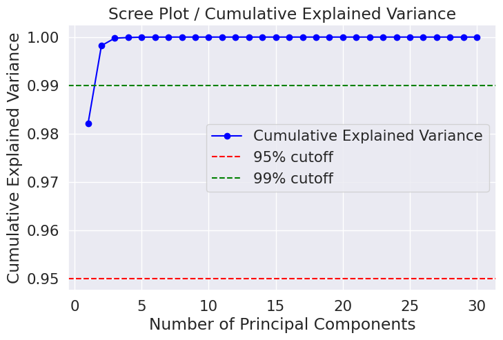
0.99941502 0.99968761 0.99991763 0.99997061 0.99999557 1. ]Cumulative explained ratio PCA FROM ORIGINAL DATA::
[0.98204467 0.99822116 0.99977867 0.9998996 0.99998788 0.99999453
0.99999854 0.99999936 0.99999971 0.99999989 0.99999996 0.99999998
0.99999999 0.99999999 1. 1. 1. 1.
1. 1. 1. 1. 1. 1.
1. 1. 1. 1. 1. 1. ]Reading the Graph: The 95% and 99% Rules
A common heuristic is to keep enough components to explain 95% or 99% of the variance. These thresholds are drawn as horizontal dashed lines on the cumulative variance plot. The point where the curve crosses the red 95% line tells you the minimum number of components needed to retain 95% of the information.
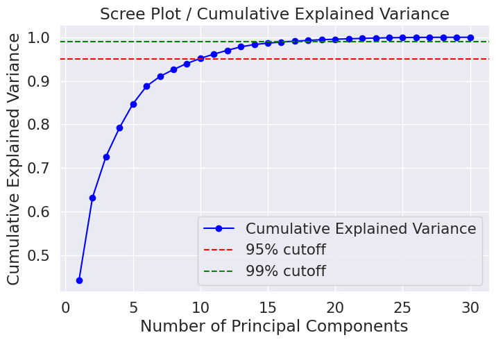
For the normalized WDBC dataset, the plot reveals that:
- Roughly 10 components capture ~95% of total variance.
- Roughly 17 components capture ~99% of total variance.
- The first 2 components alone capture a surprisingly large portion when applied to raw (non-normalized) data — because area and perimeter’s large values dominate.
!! The Subjectivity of Choosing k !!
There is no mathematically “correct” number of components. Choosing k is a trade-off between information retained and dimensionality reduced. In this project, two different choices were made: k=2 for PCA on raw data, and k=17 for PCA on normalized data. This subjectivity is intentional — it is part of the modeling process, and the scree plot is simply a visual tool to inform that decision. A practitioner with domain knowledge might make a different choice based on downstream model performance or computational constraints.
Applying PCA: Two Experiments
# PCA applied directly to raw (unnormalized) data → 2 components chosen
pca = PCA(n_components=2, random_state=2022)
pca.fit(X)
ori_pca_array = pca.transform(X)

# Create a labeled DataFrame with only PC1 and PC2
ori_pca = pd.DataFrame(data=ori_pca_array, columns=['PC1', 'PC2'])

# Split for modeling
X_train_pca, X_test_pca, Y_train_pca, Y_test_pca = train_test_split(
    ori_pca, y, test_size=0.3, random_state=2022
)
# PCA applied to StandardScaler-normalized data → 17 components (≈99% variance)
numb_pca = 17
pca = PCA(n_components=numb_pca, random_state=2022)
pca.fit(X_norm)
norm_pca_array = pca.transform(X_norm)
# Name columns PC1 through PC17
column_names = [f'PC{i+1}' for i in range(numb_pca)]
norm_pca = pd.DataFrame(data=norm_pca_array, columns=column_names)
X_train_norm_pca, X_test_norm_pca, Y_train_norm_pca, Y_test_norm_pca = train_test_split(
norm_pca, y, test_size=0.3, random_state=2022
)07 — Modeling
The Four Experiments
Each of the four models uses the same base classifier — Decision Tree — with GridSearchCV for hyperparameter tuning and 3-fold cross-validation to prevent overfitting during tuning. The grid searches over depth, leaf size, split criteria, and more.
# Hyperparameter search space — identical for all 4 models
parameters_dt = {
    "model__max_depth":         np.arange(1, 21),       # Tree depth: 1 to 20
    "model__min_samples_leaf":  np.arange(1, 101, 2),  # Leaf size: 1 to 99 (odd)
    "model__min_samples_split": np.arange(2, 11),       # Min split: 2 to 10
    "model__criterion":         ['gini', 'entropy'],    # Split quality measure
    "model__random_state":      [2022]
}
Model 1 — Decision Tree on Original Data
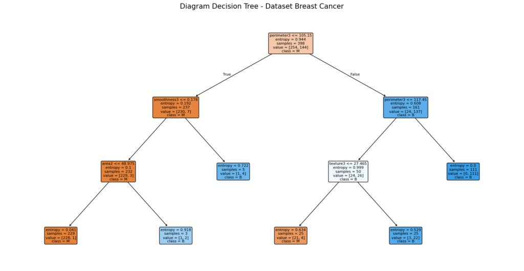
The baseline model. Raw 30-feature data is split directly into training and test sets, then fed into a Decision Tree wrapped in a scikit-learn Pipeline.
Model 01 — Original Data
# Pipeline wraps the Decision Tree (good practice — prevents leakage in CV)
classifier_dt_pipeline = Pipeline([
    ('model', DecisionTreeClassifier()),
])

ori_classifier_dt = GridSearchCV(classifier_dt_pipeline, parameters_dt, cv=3, n_jobs=-1)
ori_classifier_dt.fit(X_train, Y_train.ravel())

# Evaluate on training set
ori_y_pred_dt_train = ori_classifier_dt.predict(X_train)
ori_accuracy_dt_train = accuracy_score(Y_train, ori_y_pred_dt_train)

# Evaluate on test set
ori_y_pred_dt_test = ori_classifier_dt.predict(X_test)
ori_accuracy_dt_test = accuracy_score(Y_test, ori_y_pred_dt_test)
Model 2 — Decision Tree on Normalized Data
StandardScaler is applied to all features before splitting. The Decision Tree is then trained on the scaled features. As discussed in the StandardScaler section, this is expected to make no difference for a tree-based algorithm.
Model 02 — Normalized Data
Model 3 — Decision Tree on PCA (2 Components, Original Data)
PCA is applied directly to the raw, unnormalized data. Because features like area have enormous values compared to smoothness, the first principal component will be heavily dominated by high-scale features. Only 2 components are kept (a very aggressive reduction from 30 to 2), so there is significant information loss.
Model 03 — PCA on Original Data (k=2)
Model 4 — Decision Tree on Normalize → PCA (17 Components)
The most theoretically sound pipeline. Normalization first ensures PCA distributes importance fairly across all features. 17 components are kept — retaining approximately 99% of the dataset’s variance, reducing dimensionality by nearly half (from 30 to 17).
Model 04 — Normalize → PCA (k=17)
Evaluation Metrics
All four models are evaluated using three standard classification metrics:
| Metric | Definition | Importance in Cancer Context |
|---|---|---|
| Accuracy | (TP + TN) / Total | Overall correctness — how often the model is right. |
| Precision | TP / (TP + FP) | Of all predicted malignant cases, how many actually were? |
| Recall | TP / (TP + FN) | Of all actual malignant cases, how many did the model catch? (Clinically critical — missing a malignant tumor is dangerous.) |
In medical diagnostics, recall is often more important than accuracy or precision. A false negative (predicting Benign when it’s actually Malignant) can have life-threatening consequences, while a false positive leads to additional tests — unpleasant, but not lethal.
08 — Results
Model Performance Comparison
After running all four GridSearchCV experiments with 3-fold cross-validation and evaluating on the held-out test set, the results reveal a clear and informative pattern.
Raw 30-feature dataset, no preprocessing beyond splitting.
StandardScaler applied. All features centered and scaled to unit variance.
PCA applied directly on raw data, reduced to 2 principal components.
StandardScaler first, then PCA reducing to 17 principal components (~99% variance).
Interpreting the Results
Finding 1: Models 1 and 2 are identical. As predicted, StandardScaler has no effect on Decision Tree performance. Both models find the same optimal splits with the same accuracy, precision, and recall. This is a direct confirmation that tree-based models are scale-invariant.
Finding 2: PCA on raw data (Model 3) significantly hurts performance. Reducing to just 2 components without normalizing first is a double problem. First, those 2 components are biased toward high-variance, high-scale features. Second, two dimensions simply cannot capture the complexity of a 30-feature classification task. A drop to ~86% accuracy confirms this — the model lost too much discriminative information.
Finding 3: Normalize + PCA (Model 4) recovers most of the performance. By normalizing first and keeping 17 components (preserving ~99% variance), the model achieves ~91% test accuracy — significantly better than raw PCA, and only slightly below the full-feature models. This demonstrates that proper PCA application (normalize → then reduce) is a viable strategy that reduces dimensions from 30 to 17 with minimal information loss.
!! The Big Takeaway !!
The order of operations matters enormously in PCA pipelines. Normalize first, then PCA. Without normalization, PCA is biased and aggressive component reduction causes dramatic accuracy drops. With proper normalization, PCA can be an effective tool for creating leaner, faster models with only a modest accuracy trade-off — especially valuable when computational cost matters or when dealing with hundreds or thousands of features.
09 — Takeaways
Conclusion
This project set out to investigate how PCA — applied in different ways — changes the behavior of a Decision Tree classifier on a real medical dataset. The four experiments provide clear, interpretable answers.
✔ What Worked
- Normalize → PCA (k=17) retained ~91% accuracy while reducing features from 30 to 17
- GridSearchCV ensured fair hyperparameter comparison across all models
- Scree plots clearly visualized where the variance “knee” occurs
- The project confirmed theoretical expectations about scale-invariant classifiers
!! What to Watch Out For
- PCA on unnormalized data (Model 3, k=2) caused a significant accuracy drop
- Fitting StandardScaler on the full dataset before splitting is technically data leakage
- Choosing k is subjective — different choices lead to different accuracy trade-offs
- Decision Trees with full features tend to overfit training data (100% train accuracy)
Lessons Learned About PCA
PCA is a powerful tool, but it requires careful setup. The three most important lessons from this experiment are:
1. Always normalize before PCA. Without normalization, features with large numerical ranges dominate the principal components. The result is a biased reduction that may discard important information from small-scale features.
2. Choosing the number of components is a design decision, not a formula. The scree plot is your best tool — but where you draw the line between “enough” and “too many” depends on your use case. A 95% variance cutoff is common in practice; 99% is more conservative. In production, you’d typically validate your choice against downstream model performance.
3. PCA trades accuracy for efficiency. In this project, going from 30 features to 17 (with proper normalization) cost about 2–3% accuracy. Whether that trade-off is worth it depends on the application. For a cancer screening tool, that cost might be unacceptable. For a high-throughput pre-screening step, it might be fine.
“The best model is not always the most accurate one — it’s the one that balances accuracy, interpretability, computational cost, and the real-world stakes of its mistakes.”
Further Improvements
This experiment focused on Decision Trees, which are scale-invariant and not the ideal classifier to showcase PCA’s benefits. Future work could include:
- Using a K-Nearest Neighbors (KNN) or Support Vector Machine (SVM) classifier, where normalization and PCA can more dramatically change results.
- Using cross-validated grid search for k — treating the number of components as a hyperparameter.
- Applying proper train-only fitting of StandardScaler and PCA inside the Pipeline to eliminate data leakage.
- Examining feature contributions to principal components to understand which original features matter most.
References
- https://sebastianraschka.com/faq/docs/when-to-standardize.html ↩︎
- https://forecastegy.com/posts/do-decision-trees-need-feature-scaling-or-normalization/ ↩︎
Built with: scikit-learn · NumPy · Pandas · Matplotlib · Seaborn · Missingno · ucimlrepo
Dataset: UCI ML Repository — Wisconsin Diagnostic Breast Cancer (ID 17)
Source Code & Reproducibility
The complete codebase for this project is available on GitHub:
[GitHub Repository Link]Feel free to explore or run the project locally.
“This article was written with AI assistance for editing / drafting / translation.”


Leave a Reply