


Overview
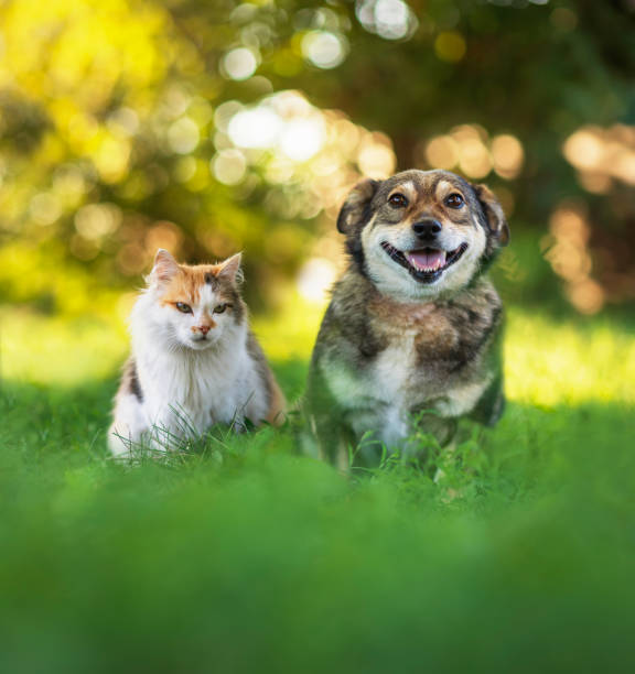
While browsing job vacancies in the data science field, I noticed that many roles — particularly around KYC (Know Your Customer) systems — involve some form of image classification. That got me thinking: when was the last time I built a classifier from the ground up? So I decided to go back to basics and build a binary image classifier the old-fashioned way — no pretrained weights, no shortcuts. Just a custom CNN trained to tell cats from dogs.
This write-up walks through the full pipeline: from data loading and augmentation, to architecture design, training strategy, evaluation, and an honest analysis of where the model falls short.
The Dataset
Two Kaggle datasets were combined for this project:
- kunalgupta2616/dog-vs-cat-images-data — used for training and validation
- tongpython/cat-and-dog — used as the held-out test set
Using separate sources for training and testing is a deliberate choice — it reduces the risk that the model is simply memorising characteristics of a single dataset’s photography style or compression artifacts. corrupted JPEG files before training to avoid silent failures downstream.
How Classification Works
Before diving into the code, here’s a quick refresher on what’s happening under the hood — the kind of thing you’d explain to a classmate before an exam.
A Convolutional Neural Network is designed to process grid-like data (images) by learning spatial patterns. Instead of looking at every pixel independently, a CNN uses small sliding windows called filters (or kernels) that scan across the image and detect local features — edges, corners, textures, and eventually higher-level shapes like ears or eyes.
Here’s the layer-by-layer logic:
Conv2D — The core workhorse. A 3×3 filter slides across the image, computing a dot product at every position. Each filter learns to detect a specific pattern. Stack 128 of them, and you get 128 different feature maps from one image.
ReLU (Rectified Linear Unit) — The activation function applied after convolution. It zeroes out any negative values, introducing non-linearity. Without it, stacking layers would just be one big linear transformation — useless for complex patterns.
MaxPooling — Downsamples the feature maps by taking the maximum value in each small region (e.g., 2×2). This reduces spatial size, cuts computation, and provides a small degree of translation invariance — the model doesn’t panic if the cat’s ear is 3 pixels to the left.
Flatten → Dense layers — Once the convolutions have extracted spatial features, the result is flattened into a 1D vector and passed through fully connected layers, which learn the final classification logic.
Sigmoid output — For binary classification, the final neuron outputs a single number between 0 and 1. Closer to 0 = Cat, closer to 1 = Dog.
Data Preprocessing
Three key hyperparameters were set upfront — grouped together deliberately so that retuning only requires changing values in one place:
batchSize = 128   # Images processed per training step
imageSize = 200   # All images resized to 200×200 pixels
epochs    = 50    # Maximum training passes
All images were resized to a uniform 200×200 RGB format. Corrupted or badly encoded files were filtered out before training began.
Data Augmentation
Augmentation artificially expands the training set by generating modified versions of existing images. The transformations used here are intentionally conservative:
dataAugmentationLayers = [
    layers.RandomFlip("horizontal"),   # Mirror the image left-right
    layers.RandomRotation(0.1),        # Rotate up to ±10% of a full turn (~36°)
    layers.RandomZoom(0.1),            # Zoom in or out by up to 10%
]
More aggressive options exist — blur, brightness shifts, noise, vertical flips — but these three are sufficient to reduce overfitting without distorting the core visual content.
Crucially, augmentation is applied only to the training set. The validation and test sets see real, unmodified images — otherwise your evaluation metrics would be meaningless.
Before feeding images into the model, all pixel values are rescaled from the [0, 255] RGB range to [0, 1]. Large input values can destabilise gradient updates during training.
layers.Rescaling(1./255)This normalization step is important because raw RGB values in the hundreds can cause large, unstable gradients early in training. Keeping inputs in a small, consistent range helps the optimizer converge faster and more smoothly.
Model Architecture
The model is a Sequential CNN with 4 convolutional blocks followed by fully connected layers:
Input: 200×200×3 RGB Image
→ Conv2D(128) + BatchNorm + ReLU + MaxPool
→ Conv2D(64) + MaxPool
→ Conv2D(64) + MaxPool
→ Conv2D(64, L1L2 Regularization) + MaxPool + BatchNorm
→ Flatten
→ Dense(512) + BatchNorm
→ Dense(512) + Dropout(0.1) + BatchNorm
→ Dense(512) + Dropout(0.2) + BatchNorm
→ Dense(1, sigmoid)  ← Output
Three regularisation techniques work in concert here:
Batch Normalisation normalises the activations within each mini-batch, keeping values in a stable range. This speeds up training and reduces sensitivity to weight initialisation.
L1L2 Regularisation adds a penalty term to the loss function proportional to the magnitude of the weights. This discourages any single weight from growing too large — the model can’t “cheat” by leaning heavily on one feature.
Dropout randomly disables a fraction of neurons during each training step. The idea is elegant: if a neuron can’t rely on its neighbours being active, it’s forced to learn independently useful representations rather than co-adapting with other neurons.
Training Strategy
Two callbacks were used to prevent overfitting and wasted compute:
ReduceLROnPlateau — monitors val_accuracy and halves the learning rate if it stops improving for 2 consecutive epochs. When a model gets close to a good solution, large update steps can cause it to overshoot. Reducing the learning rate lets it fine-tune more carefully.
EarlyStopping — halts training if val_loss doesn’t improve for 3 consecutive epochs. This prevents the classic scenario where training loss keeps falling while validation loss quietly climbs — the textbook sign of overfitting.
Results
Accuracy & Loss
| Dataset | Accuracy | Loss |
|---|---|---|
| Training | 94.22% | 0.159 |
| Validation | 94.50% | 0.151 |
| Test | 94.46% | 0.152 |
The training and validation curves track closely — no significant gap between them, which means the model generalised well rather than memorising the training data.
Confusion Matrix
| Predicted: Cat | Predicted: Dog | |
|---|---|---|
| Actual: Cat | 970 ✅ | 41 ❌ |
| Actual: Dog | 71 ❌ | 941 ✅ |
The confusion matrix gives a more granular view than accuracy alone. Out of 1,011 actual cats, 41 were misclassified as dogs. Out of 1,012 actual dogs, 71 were misclassified as cats.
From this we can derive:
- Cat Recall (Sensitivity): 970 / 1011 = 95.9% — the model correctly identifies most cats
- Dog Recall: 941 / 1012 = 93.0% — slightly lower, but still strong
- Overall Accuracy: (970 + 941) / 2023 = 94.5%
The diagonal cells (970 and 941) represent correct predictions. The off-diagonal cells represent mistakes. A perfect model would have zeros everywhere off-diagonal. This one’s close, but not quite — and the raw prediction scores tell us more about why.
The Bias Problem: When the Model Sees Dogs Everywhere
Despite the clean metrics, real-world testing revealed an uncomfortable pattern. Here are a selection of individual predictions:
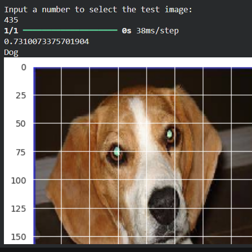
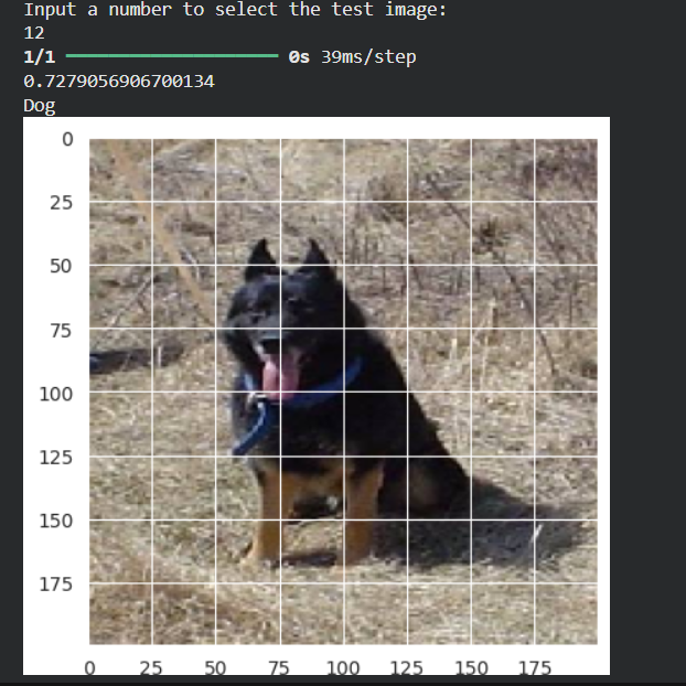
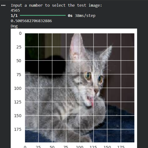
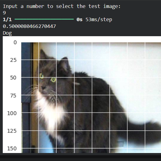
Table results from some experiments
| Image | True Label | Predicted | Score |
|---|---|---|---|
| #23 | Dog | Dog ✅ | 0.7310 |
| #12 | Dog | Dog ✅ | 0.7279 |
| #24 | Cat | Dog ❌ | 0.5180 |
| #6 | Cat | Dog ❌ | 0.5007 |
| #435 | Dog | Dog ✅ | 0.7310 |
| #11 | Cat | Dog ❌ | 0.5000 |
| #9 | Cat | Dog ❌ | 0.5001 |
| #2343 | Cat | Dog ❌ | 0.5000 |
| #4565 | Cat | Dog ❌ | 0.5006 |
The pattern is immediately clear. Dogs are predicted with genuine confidence (scores around 0.73). Cats that are misclassified all sit just above the 0.5 decision boundary — scores of 0.500, 0.501, 0.518. The model is barely calling them dogs. It’s not wrong confidently — it’s wrong hesitantly.
This tells us that the model’s internal “Cat region” in the sigmoid output space is slightly miscalibrated. The cats that the model is most unsure about are being pushed just past the 0.5 line into Dog territory.
Possible causes
- Slight class imbalance in the training data
- The model may have seen more visually varied dog images, making it harder to learn a tight dog boundary
- Certain cat poses or colorings may visually resemble dog features at 200×200 resolution
Quick Fix: Adjusting the Decision Threshold
The simplest intervention is to raise the threshold above which we call something a Dog:
print("Dog" if score >= 0.52 else "Cat")This small shift of 0.02 would correctly reclassify the borderline cats (scores of 0.50–0.52) without disrupting confident dog predictions (0.73+). It’s not a “fix” to the model’s learned weights — it’s a post-hoc calibration of the decision boundary.
This is a legitimate technique in production systems, especially when one type of error is more costly than the other (e.g., in medical imaging, you’d push thresholds differently for false positives vs. false negatives).
The proper long-term solution would be hyperparameter tuning — adjusting class weights, batch size, learning rate, or architecture — but that comes at the cost of retraining time.
What’s Next: Transfer Learning with PyTorch
Building a CNN from scratch is a great learning exercise, but modern practice leans heavily on transfer learning — taking a model pre-trained on millions of images (like ResNet, EfficientNet, or VGG) and fine-tuning it for your specific task.
The next project will explore this approach using PyTorch, which offers more flexibility in defining custom training loops, makes gradient manipulation more transparent, and is the dominant framework in research settings.
With transfer learning, even a small dataset can achieve high accuracy quickly, because the pre-trained model already “knows” low-level features like edges, textures, and shapes — you’re just teaching it what a cat vs. dog looks like at the high level.
Summary
This project covered the full pipeline of a binary image classification task:
- Dataset loading, validation, and preprocessing
- Data augmentation to improve generalization
- CNN architecture design with regularization techniques
- Smart training with callbacks
- Evaluation and honest analysis of model bias
- A lightweight fix via threshold adjustment
The 94%+ accuracy is solid for a from-scratch CNN, and the bias analysis shows that raw accuracy alone doesn’t tell the whole story — understanding where and why a model fails is just as important as the headline number.
Built with: TensorFlow 2.x · Keras · NumPy · Pandas · Matplotlib · Seaborn · scikit-learn
Dataset: Kaggle — kunalgupta2616 & tongpython
Source Code & Reproducibility
The complete codebase for this project is available on GitHub:
[GitHub Repository Link]Feel free to explore or run the project locally.
“This article was written with AI assistance for editing / drafting / translation.”


Leave a Reply