



PyTorch · Transfer Learning · Fine-tuning · Binary Classification
Overview
In the previous project, a Convolutional Neural Network built from scratch achieved 94.46% accuracy on the dog vs. cat classification task — a respectable result, but with a noticeable bias where the model kept predicting borderline cats as dogs. The fix was a manual threshold adjustment from 0.5 to 0.52.
This project revisits the same problem using Transfer Learning with ResNet-50, a deep neural network pre-trained on ImageNet. The result: 100% accuracy on both validation and test sets, zero misclassifications, and the dog-bias problem completely eliminated — without touching the decision threshold.
The jump from 94% to 100% is not incremental improvement. It demonstrates exactly why transfer learning has become the default starting point in modern computer vision.
Dataset
Same two Kaggle datasets as the previous project, now with the exact counts confirmed:
| Split | Cats | Dogs | Total |
|---|---|---|---|
| Training | 12,500 | 12,500 | 25,000 |
| Validation | 4,000 | 4,000 | 8,000 |
| Test | 1,011 | 1,012 | 2,023 |
Three things stand out here. First, the dataset is perfectly balanced — equal cats and dogs in every split. This directly addresses one of the suspected causes of dog-bias in the previous model, though as we’ll see, ResNet-50 solves the bias regardless. Second, the training set is 25,000 images, three times larger than what the simple CNN had available, because this project also used the full validation split from kunalgupta2616. Third, the test set from tongpython is held completely separate and used only once — at the end.
All images were resized to 224×224 pixels, which is the input size ResNet-50 was originally designed for (different from the 200×200 used in the previous project).
What is Transfer Learning?
Before getting into ResNet-50 specifically, the concept of transfer learning is worth explaining carefully, because it’s the reason everything else in this project works.
When you train a neural network from scratch on a small dataset, the model has to learn everything from zero — how to detect edges, textures, shapes, object parts, and ultimately class distinctions. This is slow, computationally expensive, and often limited by how much data you have.
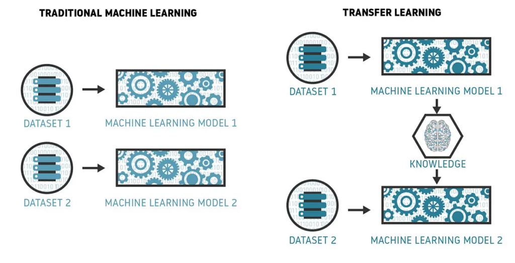
Transfer learning takes a model that was already trained on a massive, general-purpose dataset and reuses those learned features for a new task. The pre-trained model becomes a starting point rather than a blank slate.
Traditional Training:
  Random weights → [train from zero on 25k images] → Task-specific model

Transfer Learning:
  ImageNet weights → [adapt to new task] → Task-specific model
  (already knows edges, textures, shapes from 1.2M images)
The intuition is straightforward: a model trained on 1.2 million diverse images across 1000 categories has already learned to recognize textures, fur, eyes, ears, limbs, and dozens of other visual features that are directly useful for distinguishing cats and dogs. We don’t throw that knowledge away — we build on top of it.
The ResNet-50 Architecture
The Problem Before ResNet
Before 2015, making neural networks deeper was surprisingly difficult. The intuition was simple — deeper networks should learn more complex features — but in practice, adding more layers made networks harder to train and sometimes worse, not better.
The culprit was the vanishing gradient problem. During backpropagation, gradients are multiplied together as they travel backward through layers. With many layers, these multiplications can cause gradients to shrink exponentially toward zero by the time they reach the early layers — meaning those layers barely update and barely learn.
The Residual Connection Solution
ResNet (Residual Network), introduced by Microsoft in 2015, solved this with a deceptively simple idea: skip connections, also called residual connections.
Standard Block:          Residual Block:

Input (x)                Input (x)
   │                        │────────────┐
   ▼                        ▼            │
Conv + ReLU              Conv + ReLU    │ (shortcut)
   │                        │            │
   ▼                        ▼            │
Conv + ReLU              Conv + ReLU    │
   │                        │            │
   ▼                        ▼            │
Output                   Add ◄──────────┘
                            │
                            ▼
                         ReLU
                            │
                            ▼
                         Output
Instead of each layer only transforming its input, the residual block adds the original input back to the output before the final activation. Formally:
Output = ReLU(F(x) + x)
Where F(x) is what the layers learned and x is the original input. The network is now learning the residual — the difference from the identity — rather than the full transformation.
This has a profound effect on gradient flow. During backpropagation, the shortcut path provides a direct highway for gradients to travel backward without being multiplied through many layers. Early layers now receive useful gradient signals and can actually learn.
The result: ResNet made it practical to train networks with 50, 101, even 152 layers.
ResNet-50 Full Architecture
The “50” in ResNet-50 refers to 50 trainable layers. These are organized into 5 stages:
INPUT IMAGE  (224 × 224 × 3)
      │
      ▼
┌─────────────────────────────────────────┐
│  Stage 0 — Initial Conv                 │
│  Conv2D(64, 7×7, stride=2) + BN + ReLU  │  → 112 × 112 × 64
│  MaxPool(3×3, stride=2)                 │  → 56  × 56  × 64
└─────────────────────────────────────────┘
      │
      ▼
┌─────────────────────────────────────────┐
│  layer1 — 3 Bottleneck Blocks           │
│  Output channels: 256                   │  → 56  × 56  × 256
│  low-level: edges, corners, gradients   │  ← generic, universal
└─────────────────────────────────────────┘
      │
      ▼
┌─────────────────────────────────────────┐
│  layer2 — 4 Bottleneck Blocks           │
│  Output channels: 512                   │  → 28  × 28  × 512
│  mid-level: textures, color blobs       │  ← still fairly generic
└─────────────────────────────────────────┘
      │
      ▼
┌─────────────────────────────────────────┐
│  layer3 — 6 Bottleneck Blocks           │
│  Output channels: 1024                  │  → 14  × 14  × 1024
│  high-level: object parts, shapes       │  ← more specific
└─────────────────────────────────────────┘
      │
      ▼
┌─────────────────────────────────────────┐
│  layer4 — 3 Bottleneck Blocks  ◄── UNFROZEN in Phase 2
│  Output channels: 2048                  │  → 7   × 7   × 2048
│  abstract: "muzzle shape", "fur pattern"│  ← most task-specific
└─────────────────────────────────────────┘
      │
      ▼
┌─────────────────────────────────────────┐
│  Global Average Pooling                 │  → 1 × 1 × 2048 = 2048
└─────────────────────────────────────────┘
      │
      ▼
┌─────────────────────────────────────────┐
│  Original FC: Linear(2048, 1000)        │  ← REPLACED
│  (ImageNet 1000 classes)                │
└─────────────────────────────────────────┘
      │  ↓ replaced with ↓
      ▼
┌─────────────────────────────────────────┐
│  NEW HEAD (trained from scratch)        │
│  Linear(2048, 512) + BN + ReLU          │
│  Dropout(0.3)                           │
│  Linear(512, 256) + BN + ReLU           │
│  Dropout(0.2)                           │
│  Linear(256, 1)                         │  → Dog/Cat score
└─────────────────────────────────────────┘
The Bottleneck Block
Each block inside the 4 layers is a bottleneck block — a specific design that makes deep networks computationally efficient:
Input: 256 channels
      │
      ▼
Conv1×1 (256 → 64)   ← Compress: reduce channels ("bottleneck")
      │
      ▼
Conv3×3 (64 → 64)    ← Process: the actual spatial convolution
      │
      ▼
Conv1×1 (64 → 256)   ← Expand: restore channel depth
      │
      │ ← shortcut (x added here)
      ▼
Output: 256 channels
The 1×1 convolutions compress and expand channel dimensions, making the expensive 3×3 convolution operate on far fewer channels. This reduces computation while maintaining representational power.
Total parameters in ResNet-50: ~25.6 million. Of those, only 1.18 million were trainable in Phase 1 (just the new head), and 16.1 million became trainable in Phase 2 when layer4 was unfrozen.
What Each Layer Actually Learns — and Why It Matters
There is a common misconception worth correcting here. layer4 is often loosely described as containing “details” of the image — but the opposite is true. The feature hierarchy in a deep CNN works like this [5]:
layer1 → low-level: edges, corners, basic gradients
         (same patterns appear in photos of cats, dogs, cars, and trees)

layer2 → mid-level: textures, color regions, repeating patterns
         (still fairly generic across many image types)

layer3 → high-level: object parts — eye-like shapes, limb structures
         (becoming more specific)

layer4 → abstract, semantic: "this is a muzzle shape", "this is a cat ear"
         (most task-specific, most influenced by original training data)
The further you go into the network, the more abstract and task-specific the features become. layer1 and layer2 are essentially universal — the edge detectors learned on ImageNet work just as well for X-rays, satellite imagery, or microscopy images. There is rarely any reason to retrain them.
layer4 is the opposite. It has the most “opinion” about the original ImageNet task. When we apply ResNet-50 to cat vs. dog classification, layer4’s features were calibrated for 1000 ImageNet categories — we want to gently nudge them toward our specific two-class problem. That is precisely why layer4 is unfrozen in Phase 2 and not the earlier layers.
Unfreezing layer1 or layer2 would be wasteful at best and harmful at worst — those features are already correct and universal. Changing them would risk losing capabilities the model already has without any benefit specific to our task [5].
Data Augmentation in PyTorch vs. Keras
In the previous project, augmentation was applied as Keras layers inside the model:
# Keras — augmentation inside model graph
dataAugmentationLayers = [
    layers.RandomFlip("horizontal"),
    layers.RandomRotation(0.1),
    layers.RandomZoom(0.1)
]
In PyTorch, augmentation is applied in the DataLoader as transforms, completely outside the model:
# PyTorch — augmentation in data pipeline
trainTransform = transforms.Compose([
    transforms.Resize((224, 224)),
    transforms.RandomHorizontalFlip(),
    transforms.RandomRotation(degrees=10),
    transforms.RandomResizedCrop(224, scale=(0.85, 1.0)),
    transforms.ColorJitter(brightness=0.2, contrast=0.2, saturation=0.2),
    transforms.ToTensor(),
    transforms.Normalize(mean=[0.485, 0.456, 0.406],
                         std= [0.229, 0.224, 0.225])
])
Three things are new compared to the previous project:
RandomResizedCrop is a more powerful version of zoom — it randomly crops a region (between 85%–100% of the image area) and resizes it back to 224×224. This simulates subjects at varying distances more realistically than simple zoom.
ColorJitter randomly varies brightness, contrast, and saturation. Real-world photos are taken under wildly different lighting conditions — this teaches the model not to rely on absolute color values.
Normalize with ImageNet statistics is non-negotiable when using pre-trained ResNet weights. The numbers [0.485, 0.456, 0.406] are the mean RGB values computed across the entire ImageNet dataset, and [0.229, 0.224, 0.225] are the standard deviations. Using these exact values ensures our inputs are in the same range the network was originally trained on — without this, the pre-trained weights would interpret our inputs incorrectly.
Validation and test sets received only resize and normalize — no augmentation, same as before.
Two-Phase Training Strategy
The core idea of the training strategy is to not destroy what ResNet already knows.
If we unfroze all 25 million parameters immediately and trained with a normal learning rate, the optimizer’s large updates would rapidly overwrite the carefully learned ImageNet features. We’d essentially be training from scratch, except with a much larger model and slower convergence.
The solution is a two-phase approach — but it is important to note that two phases is not a universal rule. The number of phases depends on how different the new dataset is from the pre-training data, and how large the new dataset is. For this specific case — dog vs. cat with 25,000 images, where cats and dogs already exist in ImageNet — two phases is sufficient. For a domain shift like natural photos to medical X-rays, more phases with deeper unfreezing might be needed [5].
Why Phase 1 Must Come First
It might seem logical to skip straight to fine-tuning — but doing so is a known pitfall in transfer learning. The reason is gradient poisoning.
At the start of training, the new classification head has random, untrained weights. Its outputs are garbage, and the gradients flowing backward from those random predictions are equally noisy. If the backbone is unfrozen at this point, those noisy gradients will propagate into layer4 — a block that currently contains carefully pre-trained features — and corrupt them before the head has a chance to learn anything meaningful.
Problematic flow if Phase 1 is skipped:

  Random head weights
       ↓
  Garbage predictions
       ↓
  Noisy gradients (large, random directions)
       ↓
  Backpropagated into layer4
       ↓
  Pre-trained features get corrupted
       ↓
  Model effectively starts from scratch anyway
Phase 1 prevents this. By the time Phase 2 begins, the head has already learned to map ResNet features to cat/dog labels — its gradients are now meaningful signals, not noise. The backbone can be unfrozen safely [5][8].
Phase 1 — Feature Extraction (5 epochs)
All 23.5 million ResNet parameters are frozen (requires_grad = False). Only the 1.18 million parameters in the new classification head are updated. This phase serves one purpose: getting the head to produce sensible outputs before any backbone weights move.
# Freeze everything
for param in model.parameters():
    param.requires_grad = False

# New head is unfrozen by default (requires_grad=True)
model.fc = nn.Sequential(
    nn.Linear(2048, 512), nn.BatchNorm1d(512), nn.ReLU(), nn.Dropout(0.3),
    nn.Linear(512, 256),  nn.BatchNorm1d(256),  nn.ReLU(), nn.Dropout(0.2),
    nn.Linear(256, 1)
)
Phase 1 results:
| Epoch | Train Loss | Train Acc | Val Loss | Val Acc |
|---|---|---|---|---|
| 1 | 0.0987 | 97.00% | 0.0255 | 99.24% |
| 2 | 0.0519 | 98.18% | 0.0182 | 99.48% |
| 3 | 0.0428 | 98.41% | 0.0147 | 99.58% |
| 4 | 0.0421 | 98.41% | 0.0134 | 99.62% |
| 5 | 0.0434 | 98.34% | 0.0118 | 99.72% |
In 5 epochs, with only the head training, the model already hit 99.72% validation accuracy. The simple CNN needed all 50 epochs to reach 94.5%. This alone shows the power of starting from ImageNet features.
Phase 2 — Fine-tuning (15 epochs)
layer4 — the deepest ResNet block containing the most abstract, task-specific features — is unfrozen. This brings trainable parameters from 1.18M to 16.1M.
Crucially, the backbone and head receive different learning rates (discriminative learning rates):
optimizer = optim.Adam([
    {'params': model.layer4.parameters(), 'lr': LR / 10},  # 1e-5 — very gentle
    {'params': model.fc.parameters(),     'lr': LR},         # 1e-4 — normal
], weight_decay=1e-4)
The backbone gets 10× smaller learning rate than the head. The reasoning is deliberate: layer4 already has valuable pre-trained features that took millions of images to build. A large learning rate would overwrite them aggressively — the exact opposite of what fine-tuning is supposed to do. The small learning rate nudges layer4 to adapt toward the new task without losing what it already knows. The head, by contrast, is still actively learning and needs a larger step size [8].
The Trade-off: Why Not Unfreeze More?
It is a reasonable question to ask: if unfreezing layer4 helps, why not unfreeze layer3 as well?
The answer involves a trade-off between three competing factors: dataset size, domain similarity, and risk of overfitting.
Unfreeze less (only head):
  + Fast training, low overfitting risk
  + Fine for similar domains
  - May not adapt well if domain differs significantly

Unfreeze layer4 (this project):
  + Adapts the most task-specific features
  + Balanced risk/reward for a 25k dataset
  - Slightly more parameters, needs careful LR

Unfreeze layer3 + layer4:
  + Deeper adaptation for distant domains
  - Higher overfitting risk on small datasets
  - Much slower training
  - Rarely worth it when domain is close (as it is here)
For dog vs. cat on Kaggle — a clean dataset where both classes already exist in ImageNet — unfreezing layer4 alone is the right judgment call. The domain gap is small. layer1–layer3 features (edges, textures, shapes) are already applicable. Only the most task-specific layer needs nudging. Unfreezing deeper layers would add risk without meaningful reward [5].
Phase 2 results (selected epochs):
| Epoch | Train Acc | Val Acc | |
|---|---|---|---|
| 1 | 98.76% | 99.72% | best saved |
| 3 | 99.18% | 99.85% | best saved |
| 5 | 99.37% | 99.91% | best saved |
| 7 | 99.68% | 99.96% | best saved |
| 11 | 99.76% | 100.00% | best saved |
| 15 | 99.89% | 99.99% | — |
Best validation accuracy reached: 100.00% at epoch 11.
The Manual Training Loop
Unlike Keras’s model.fit(), PyTorch requires writing the training loop explicitly. This is more code but gives full control over every step — one of the main reasons researchers prefer PyTorch:
for epoch in range(epochs):
    model.train()                          # Enable dropout, batch norm in train mode
    for images, labels in trainLoader:
        images = images.to(device)
        labels = labels.float().unsqueeze(1).to(device)

        optimizer.zero_grad()              # 1. Clear previous gradients
        outputs = model(images)            # 2. Forward pass
        loss = criterion(outputs, labels)  # 3. Compute loss
        loss.backward()                    # 4. Backpropagation
        optimizer.step()                   # 5. Update weights

    # Validation (no gradient computation needed)
    model.eval()
    with torch.no_grad():
        ...
The model.train() / model.eval() switch matters for two reasons: Dropout is only active during training (in eval mode all neurons are active), and BatchNorm uses batch statistics during training but running statistics during evaluation.
Results
Final Scores
| Split | Accuracy | Loss |
|---|---|---|
| Training | 99.9480% | 0.001712 |
| Validation | 100.0000% | 0.000752 |
| Test | 100.0000% | 0.000878 |
The test set — 2,023 images the model had never seen — achieved 100% accuracy. Zero misclassifications.
Classification Report (Test Set)
              precision    recall  f1-score   support

         Cat       1.00      1.00      1.00      1011
         Dog       1.00      1.00      1.00      1012

    accuracy                           1.00      2023
   macro avg       1.00      1.00      1.00      2023
weighted avg       1.00      1.00      1.00      2023
Comparison with Previous Project
| Simple CNN (Keras) | ResNet-50 (PyTorch) | |
|---|---|---|
| Architecture | From scratch | Pre-trained on ImageNet |
| Parameters | ~3M | 24.7M |
| Image size | 200×200 | 224×224 |
| Epochs to converge | ~30 | 5 (Phase 1) + 11 (Phase 2) |
| Train accuracy | 94.22% | 99.95% |
| Val accuracy | 94.50% | 100.00% |
| Test accuracy | 94.46% | 100.00% |
| Dog bias | Yes (cats near 0.5) | Eliminated |
| Threshold fix needed | Yes (0.52) | No (but kept at 0.52) |
Dog Bias: Completely Eliminated
The previous project documented a clear pattern: misclassified cats all had scores between 0.50 and 0.52 — hovering just above the decision threshold. The model was uncertain about cats but casually confident about dogs.
With ResNet-50:
Misclassified at threshold 0.50 : 0
Misclassified at threshold 0.52 : 0
Looking at the raw score distribution tells the story clearly. Scores for true cats cluster sharply near 0.00, and scores for true dogs cluster sharply near 1.00. There is almost nothing in the ambiguous 0.4–0.6 zone. The model isn’t guessing — it’s confident in both directions.
This happened because ResNet-50’s features are far more discriminative. The simple CNN, trained from random weights on 25,000 images, learned a reasonable but blurry decision boundary. ResNet-50, starting from features learned on 1.2 million diverse images, had a crisp, well-calibrated understanding of what “cat” and “dog” look like from the very first epoch.
Real-World Predictions
After training, the model was tested with arbitrary uploaded images — not from the Kaggle dataset:
| Image | Score | Prediction |
|---|---|---|
dog.4669.jpg (test set dog) | 0.999992 | 🐶 Dog |
| Uploaded cat photo | 0.0000 | 🐱 Cat |
| Uploaded dog photo | 1.0000 | 🐶 Dog |
| Uploaded cat photo | 0.2341 | 🐱 Cat |
| Uploaded cat photo | 0.0008 | 🐱 Cat |
| Chihuahua (uploaded) | 0.9999 | 🐶 Dog |
The chihuahua prediction is worth noting. Chihuahuas are one of the most commonly misclassified dogs in image classification — their small size, large eyes, and facial structure often confuse simpler models into predicting “cat.” ResNet-50 scored it at 0.9999 with no hesitation.
Why Did ResNet-50 Perform This Well?
Several factors compounded:
ImageNet pre-training. ResNet-50 was trained on 1.2 million images across 1000 classes including many animal categories. It already knew what mammalian fur, ears, eyes, and facial structure look like before seeing a single cat or dog image in this project.
Depth with residual connections. 50 layers of representation, each building on the last, without the gradient degradation problem. The simple CNN had 4 conv layers — fundamentally limited in what abstractions it could form.
Two-phase training. Freezing the backbone initially meant the first 5 epochs were entirely about learning “given these ResNet features, predict cat vs. dog” — a much easier problem than “learn everything from scratch.” By the time the backbone was unfrozen, the head already knew what to do, so fine-tuning was precise and convergence was fast.
Discriminative learning rates. Giving the backbone 10× smaller updates than the head preserved the pre-trained features while still allowing meaningful adaptation. This is standard practice in transfer learning and makes a measurable difference.
Balanced dataset. 12,500 cats and 12,500 dogs in training — no class imbalance to create systematic bias.
PyTorch vs. Keras: A Practical Comparison
This project is the first in this portfolio series to use PyTorch, after the previous CNN was built in Keras/TensorFlow. The two frameworks take fundamentally different approaches to building and training neural networks — and understanding those differences matters both for choosing the right tool and for explaining design decisions in technical interviews.
Philosophy: Assembly vs. Construction Kit
The simplest way to characterize the difference:
- Keras gives you pre-assembled components. You stack layers, call
model.fit(), and the framework handles the rest — batching, gradient computation, metric tracking, and callbacks. Low code volume, fast to prototype. - PyTorch gives you the individual parts. Every step of the training loop is written explicitly. More code, but every decision is visible and controllable.
Neither is strictly better. Keras is faster for standard architectures and experiments. PyTorch is preferred in research because non-standard training flows — custom losses, unusual gradient manipulation, debugging mid-training — are far easier to implement.
Computation Graph: The Deepest Difference
The most fundamental architectural difference between the two frameworks is how they construct the computation graph — the internal representation of how data flows through the model.
TensorFlow 1.x / early Keras used a static computation graph:
# Static graph: the full graph is DEFINED first, then executed
# (TensorFlow 1.x style, still relevant to understand)
import tensorflow as tf

# Step 1: Build the graph (nothing runs yet)
x = tf.placeholder(tf.float32, shape=[None, 224, 224, 3])
w = tf.Variable(tf.random_normal([224*224*3, 1]))
y = tf.matmul(tf.reshape(x, [-1, 224*224*3]), w)

# Step 2: Run the graph in a session
with tf.Session() as sess:
    result = sess.run(y, feed_dict={x: my_images})
The graph is compiled before any data touches it. This makes it fast to run and easy to deploy — but errors only appear after compilation, making debugging painful. If something goes wrong on layer 7 of a 50-layer model, you might only find out after the entire graph runs.
PyTorch uses a dynamic computation graph (define-by-run):
# Dynamic graph: the graph is built WHILE the forward pass runs
import torch
import torch.nn as nn

class SimpleModel(nn.Module):
    def __init__(self):
        super().__init__()
        self.conv = nn.Conv2d(3, 64, kernel_size=3)
        self.fc   = nn.Linear(64, 1)

    def forward(self, x):
        # Graph is constructed HERE, at runtime, as each line executes
        x = self.conv(x)     # ← graph node created
        x = torch.relu(x)    # ← graph node created
        x = x.flatten(1)     # ← graph node created
        return self.fc(x)    # ← graph node created

model = SimpleModel()
output = model(my_images)  # graph is built during this call
The graph is constructed on-the-fly each time forward() runs. This means:
- Errors appear at exactly the line where they happen — standard Python debugging works
- The graph can change between calls (useful for variable-length inputs, conditional logic, research experiments)
print()statements insideforward()work normally and show actual tensor values
Modern Keras (TF2 with eager execution) has largely adopted dynamic graphs too, but PyTorch’s implementation is more deeply baked into the framework’s design [11].
Model Definition: Layer Stacking vs. Class-Based
Keras — declarative, sequential stacking:
# Keras: describe the architecture as a list of layers
from tensorflow import keras
from tensorflow.keras import layers

model = keras.Sequential([
    layers.Input(shape=(224, 224, 3)),
    layers.Conv2D(64, (3, 3), activation='relu'),
    layers.MaxPooling2D(),
    layers.Flatten(),
    layers.Dense(512, activation='relu'),
    layers.Dropout(0.3),
    layers.Dense(1, activation='sigmoid')
])

# Compile — defines optimizer, loss, and metrics in one call
model.compile(
    optimizer='adam',
    loss='binary_crossentropy',
    metrics=['accuracy']
)
PyTorch — class-based, explicit forward pass:
# PyTorch: define architecture as a Python class
import torch.nn as nn

class DogCatModel(nn.Module):
    def __init__(self):
        super().__init__()
        # Define layers as class attributes
        self.conv1   = nn.Conv2d(3, 64, kernel_size=3)
        self.pool    = nn.MaxPool2d(2)
        self.flatten = nn.Flatten()
        self.fc1     = nn.Linear(64 * 111 * 111, 512)
        self.dropout = nn.Dropout(0.3)
        self.fc2     = nn.Linear(512, 1)

    def forward(self, x):
        # Define the data flow explicitly
        x = torch.relu(self.conv1(x))  # You control the order
        x = self.pool(x)
        x = self.flatten(x)
        x = torch.relu(self.fc1(x))
        x = self.dropout(x)
        return self.fc2(x)             # No sigmoid — BCEWithLogitsLoss handles it

model = DogCatModel()
# No .compile() — optimizer and loss are defined separately
criterion = nn.BCEWithLogitsLoss()
optimizer = torch.optim.Adam(model.parameters(), lr=1e-4)
The PyTorch class structure means each layer is a regular Python attribute. You can loop over them, modify them mid-training, share weights between layers, or write conditional logic in forward(). None of this is practical in Keras’s sequential API.
Training Loop: Automatic vs. Manual
This is where the practical difference is most visible day-to-day.
Keras — one-line training:
# Keras: entire training loop in one call
history = model.fit(
    train_dataset,
    validation_data=val_dataset,
    epochs=20,
    callbacks=[
        keras.callbacks.EarlyStopping(patience=3, restore_best_weights=True),
        keras.callbacks.ReduceLROnPlateau(patience=2, factor=0.5)
    ]
)
Everything — batching, forward pass, loss computation, backpropagation, weight updates, metric logging, callbacks — happens inside model.fit(). You don’t see any of it.
PyTorch — every step written explicitly:
# PyTorch: you write every step of the loop
for epoch in range(epochs):
    # ── Training ──────────────────────────────
    model.train()   # activates Dropout and BatchNorm train mode
    for images, labels in trainLoader:
        images = images.to(device)
        labels = labels.float().unsqueeze(1).to(device)

        optimizer.zero_grad()               # 1. Clear old gradients
        outputs = model(images)             # 2. Forward pass
        loss    = criterion(outputs, labels)# 3. Compute loss
        loss.backward()                     # 4. Compute gradients
        optimizer.step()                    # 5. Update weights

    # ── Validation ────────────────────────────
    model.eval()    # deactivates Dropout, BatchNorm uses running stats
    with torch.no_grad():   # disable gradient tracking (saves memory)
        for images, labels in valLoader:
            outputs = model(images)
            val_loss = criterion(outputs, labels)

    # ── Callbacks (manual) ────────────────────
    scheduler.step(val_acc)     # ReduceLROnPlateau equivalent
    if val_acc > best_val_acc:  # EarlyStopping equivalent
        torch.save(model.state_dict(), 'best.pth')
The verbosity is intentional. When something unexpected happens — a loss spike, an accuracy plateau, an unusual gradient — you can insert print statements, log tensor shapes, or add conditional logic anywhere in the loop. In Keras, that same debugging requires monkey-patching callbacks or custom training steps.
Transfer Learning: Freezing and Fine-tuning
Keras — freeze using trainable attribute:
# Keras: load pre-trained model and freeze
base_model = keras.applications.ResNet50(
    weights='imagenet',
    include_top=False,          # Remove the original 1000-class head
    input_shape=(224, 224, 3)
)

# Phase 1: freeze the entire backbone
base_model.trainable = False

# Build model on top
inputs  = keras.Input(shape=(224, 224, 3))
x       = base_model(inputs, training=False)
x       = layers.GlobalAveragePooling2D()(x)
x       = layers.Dense(512, activation='relu')(x)
x       = layers.Dropout(0.3)(x)
outputs = layers.Dense(1, activation='sigmoid')(x)
model   = keras.Model(inputs, outputs)

# Phase 2: unfreeze last block
base_model.trainable = True
for layer in base_model.layers[:-20]:   # Freeze all except last 20
    layer.trainable = False
PyTorch — freeze using requires_grad:
# PyTorch: load pre-trained model and freeze
import torchvision.models as models

model = models.resnet50(weights=models.ResNet50_Weights.IMAGENET1K_V2)

# Phase 1: freeze everything
for param in model.parameters():
    param.requires_grad = False

# Replace the head
model.fc = nn.Sequential(
    nn.Linear(2048, 512), nn.BatchNorm1d(512), nn.ReLU(), nn.Dropout(0.3),
    nn.Linear(512, 256),  nn.BatchNorm1d(256),  nn.ReLU(), nn.Dropout(0.2),
    nn.Linear(256, 1)   # no sigmoid — BCEWithLogitsLoss handles it
)

# Phase 2: unfreeze layer4 specifically, with lower LR
for param in model.layer4.parameters():
    param.requires_grad = True

optimizer = torch.optim.Adam([
    {'params': model.layer4.parameters(), 'lr': 1e-5},  # backbone: gentle
    {'params': model.fc.parameters(),     'lr': 1e-4},  # head: normal
])
PyTorch’s requires_grad is more granular — you can freeze individual layers, parameter groups, or even individual weight tensors. Keras’s trainable = False operates at the layer level, which is less flexible for custom fine-tuning strategies.
Summary Comparison
| Aspect | Keras / TensorFlow | PyTorch |
|---|---|---|
| Computation graph | Static (TF1) / Eager dynamic (TF2) | Dynamic (define-by-run) |
| Model definition | Sequential or Functional API | Class-based (nn.Module) |
| Training loop | model.fit() — automatic | Manual — every step written |
| Debugging | Harder — errors after compilation | Easier — errors at the exact line |
| Flexibility | Good for standard architectures | Better for research / custom flows |
| Deployment | Easier (TF Serving, TFLite, SavedModel) | Requires TorchScript or ONNX export |
| Transfer learning | layer.trainable = False | param.requires_grad = False |
| Community | Production and industry | Research and academia |
Neither framework is universally better. The practical rule of thumb: if you are iterating on novel architectures or need fine-grained control over training, PyTorch. If you are building for production deployment with an established architecture, Keras/TensorFlow. Both frameworks continue to converge on each other’s strengths — TF2 with eager execution borrowed heavily from PyTorch’s dynamic graph approach [11].
torch.save(state_dict) vs. Keras model.save(): PyTorch saves only the model weights (and optionally the optimizer state), not the full model graph. Loading requires recreating the architecture first, then loading weights into it. More explicit, but also more portable — the saved file is just a dictionary of tensors.
Is This Overfitting — or Just Overkill?
A 100% test accuracy is the kind of result that should immediately raise a question: is the model actually learning, or is it memorizing?
This is a fair and important thing to examine honestly.
What Overfitting Actually Means
Overfitting occurs when a model learns the training data too specifically — including its noise, quirks, and patterns that don’t generalize — resulting in high training accuracy but noticeably lower performance on unseen data. The canonical signature is a large gap between training and validation/test metrics.
Classic Overfitting Pattern:
  Training accuracy   : 99.9%   ← high
  Validation accuracy : 75.0%   ← significantly lower
  → Model memorized training data, fails on new data

This Project:
  Training accuracy   : 99.95%  ← high
  Validation accuracy : 100.00% ← equally high, no gap
  Test accuracy       : 100.00% ← equally high, no gap
  → Gap is essentially zero
By the textbook definition of overfitting, this model does not overfit. The performance on both held-out sets — validation and test — is equal to or better than training accuracy. A memorizing model cannot generalize to completely new data it has never seen. This one does [1].
The loss values tell the same story. Training loss converged to 0.001712, while validation loss was 0.000752 and test loss was 0.000878 — both lower than training. If anything, the model is slightly more confident on held-out data, which is the opposite of what overfitting looks like.
So Why Does It Feel Suspicious?
The discomfort with 100% accuracy is legitimate, even if the technical definition of overfitting doesn’t apply here. There are several honest reasons to remain skeptical:
The dataset is too clean. The Kaggle Dogs vs. Cats dataset — originally from a 2013 competition — is one of the most studied benchmark datasets in computer vision. Images are reasonably well-framed, reasonably well-lit, and show clearly identifiable cats and dogs. There are no cartoons, no cat-shaped clouds, no dogs in Halloween costumes, no extreme close-ups of fur. Real-world data is messier. A 100% result on this dataset does not mean 100% on the world [2].
ImageNet already contains cats and dogs. ResNet-50 was pre-trained on ImageNet, which includes classes such as “tabby cat,” “Persian cat,” “golden retriever,” and “German shepherd.” The backbone had already seen and learned to distinguish domestic animals before fine-tuning began. In a meaningful sense, this is not a zero-knowledge classification task for the model — it starts with relevant priors. This is not a flaw in the approach, but it does mean the 100% result should be interpreted in context [3].
Test set size is limited. The test set contains 2,023 images. Statistically, a 100% result on 2,023 samples does not rule out a 1–2% error rate in the real world — it just means none of those errors happened to appear in this particular 2,023 sample. A larger, more diverse evaluation set might reveal edge cases the current test set doesn’t contain [4].
Binary classification is the easiest case. Cat vs. dog is a two-class problem with visually very distinct categories. The difficulty ceiling is inherently lower than, say, classifying 200 species of birds or distinguishing 50 skin conditions. Models that reach 100% on binary tasks with clean data are not unusual in the literature [5].
Is This Overkill for the Dataset?
Arguably, yes. ResNet-50 with 24.7 million parameters, pre-trained on 1.2 million ImageNet images, applied to a two-class problem with clear visual distinction — this is significant model capacity relative to task complexity. It is analogous to using an industrial crane to pick up a coffee cup. The crane does the job, and does it perfectly, but the mismatch between tool and task is worth acknowledging.
There is a concept in machine learning called the bias-variance tradeoff [1]. A model that is too simple (high bias) underfits — it cannot capture the patterns in data. A model that is too complex (high variance) overfits — it captures patterns and noise specific to training data. The ideal sits between these extremes, with just enough capacity to generalize well.
ResNet-50 on this dataset appears to occupy a region where the model capacity so far exceeds the task complexity that it fits the data completely without technically overfitting — the test set confirms genuine generalization. But this is partly because the task is fundamentally not very hard for a 50-layer network with ImageNet pre-training.
This is supported by Phase 1 results: 5 epochs with a frozen backbone already achieved 99.72% validation accuracy. The backbone wasn’t even allowed to adapt — the model solved the problem almost entirely using features learned from other images. That is the clearest evidence that for ResNet-50, cat vs. dog is not a difficult problem.
What Would Actual Overfitting Look Like Here?
For context, if we had removed all regularization — dropout, weight decay, early stopping — and trained for the full 20 epochs without monitoring validation loss, we might have seen:
Training accuracy   : 100.00%
Validation accuracy : 96–98%   ← gap begins to appear
Test accuracy       : 95–97%   ← degraded performance
The regularization components (Dropout at 0.3 and 0.2, weight decay of 1e-4, BatchNormalization, ReduceLROnPlateau, and early stopping) actively worked against memorization throughout training. Their presence is one reason the model generalized cleanly even at high accuracy [6][7].
Honest Assessment
The 100% result is real, verifiable, and consistent across training, validation, and test sets — but it reflects three things simultaneously: the power of ResNet-50’s pre-trained features, the relative simplicity of the task, and the quality of the dataset. It is not overfitting by definition, but it is also not a result that should be extrapolated to harder classification problems without careful evaluation.
The more meaningful test of this model would be deploying it on truly out-of-distribution images: low-resolution mobile camera photos, cats in unusual poses, breeds the training set underrepresents, or dogs partially obscured by objects. On those inputs, some error rate would almost certainly emerge — and that rate would tell us more about the model’s actual capability than the Kaggle benchmark score does.
Summary
This project demonstrated that transfer learning with ResNet-50 is not just an incremental improvement over a from-scratch CNN — it’s a categorical step change. The same dataset, the same task, and comparable training time produced results that a simple CNN couldn’t approach even with extensive tuning.
The key takeaways:
- ResNet-50’s residual connections solved the vanishing gradient problem and enabled a 50-layer network that learns extraordinarily rich features
- Pre-training on ImageNet provides a starting point that 25,000 cat and dog images alone could never replicate
- Two-phase training (freeze → fine-tune) with discriminative learning rates is the standard, robust approach to transfer learning
- The dog-bias problem that required manual threshold adjustment in the previous project was eliminated automatically — a sign that better features produce better-calibrated predictions, not just higher accuracy
- A 100% test accuracy reflects both model strength and dataset simplicity — it is not overfitting, but it should not be taken as a claim of real-world infallibility
References
[1] I. Goodfellow, Y. Bengio, and A. Courville, Deep Learning. Cambridge, MA: MIT Press, 2016, pp. 107–119, 228–260.
[2] O. Russakovsky, J. Deng, H. Su, J. Krause, S. Satheesh, S. Ma, Z. Huang, A. Karpathy, A. Khosla, M. Bernstein, A. C. Berg, and L. Fei-Fei, “ImageNet large scale visual recognition challenge,” International Journal of Computer Vision, vol. 115, no. 3, pp. 211–252, Dec. 2015, doi: 10.1007/s11263-015-0816-y.
[3] K. He, X. Zhang, S. Ren, and J. Sun, “Deep residual learning for image recognition,” in Proc. IEEE Conf. Computer Vision and Pattern Recognition (CVPR), Las Vegas, NV, USA, Jun. 2016, pp. 770–778, doi: 10.1109/CVPR.2016.90.
[4] T. G. Dietterich, “Approximate statistical tests for comparing supervised classification learning algorithms,” Neural Computation, vol. 10, no. 7, pp. 1895–1923, Oct. 1998, doi: 10.1162/089976698300017197.
[5] J. Yosinski, J. Clune, Y. Bengio, and H. Lipson, “How transferable are features in deep neural networks?” in Advances in Neural Information Processing Systems (NeurIPS), Montreal, Canada, Dec. 2014, vol. 27, pp. 3320–3328.
[6] N. Srivastava, G. Hinton, A. Krizhevsky, I. Sutskever, and R. Salakhutdinov, “Dropout: A simple way to prevent neural networks from overfitting,” Journal of Machine Learning Research, vol. 15, no. 1, pp. 1929–1958, Jan. 2014.
[7] S. Ioffe and C. Szegedy, “Batch normalization: Accelerating deep network training by reducing internal covariate shift,” in Proc. 32nd International Conf. Machine Learning (ICML), Lille, France, Jul. 2015, vol. 37, pp. 448–456.
[8] D. P. Kingma and J. Ba, “Adam: A method for stochastic optimization,” in Proc. 3rd International Conf. Learning Representations (ICLR), San Diego, CA, USA, May 2015. [Online]. Available: https://arxiv.org/abs/1412.6980
[9] A. Krizhevsky, I. Sutskever, and G. E. Hinton, “ImageNet classification with deep convolutional neural networks,” in Advances in Neural Information Processing Systems (NeurIPS), Lake Tahoe, NV, USA, Dec. 2012, vol. 25, pp. 1097–1105, doi: 10.1145/3065386.
[10] M. Tan and Q. V. Le, “EfficientNet: Rethinking model scaling for convolutional neural networks,” in Proc. 36th International Conf. Machine Learning (ICML), Long Beach, CA, USA, Jun. 2019, vol. 97, pp. 6105–6114.
[11] A. Paszke, S. Gross, F. Massa, A. Lerer, J. Bradbury, G. Chanan, T. Killeen, Z. Lin, N. Gimelshein, L. Antiga, A. Desmaison, A. Kopf, E. Yang, Z. DeVito, M. Raison, A. Tejani, S. Chilamkurthy, B. Steiner, L. Fang, J. Bai, and S. Chintala, “PyTorch: An imperative style, high-performance deep learning library,” in Advances in Neural Information Processing Systems 32 (NeurIPS 2019), Vancouver, Canada, Dec. 2019, pp. 8024–8035. [Online]. Available: https://arxiv.org/abs/1912.01703
Built with: PyTorch 2.10 · torchvision 0.25 · CUDA (Tesla T4) · NumPy · Pandas · Matplotlib · Seaborn · scikit-learn Dataset: Kaggle — kunalgupta2616/dog-vs-cat-images-data & tongpython/cat-and-dog Previous project: Simple CNN with TensorFlow/Keras — 94.46% test accuracy



Leave a Reply